


Ryan Day and Brian Billick on Building an Offense and Game Planning

Ryan Day made arguably the biggest assistant hire of the off season this year when he brought in his mentor Chip Kelly to be the offensive coordinator at Ohio State. Despite a stellar 56-8 record as the head coach of the Buckeyes, Day is on the hot seat after 3 straight losses to Michigan. There is a feeling in Columbus that a seasoned offensive guru like Kelly might be the missing piece the Buckeyes need to help Day finally get over the hump against their rival and secure his job. Kelly’s expertise in the spread run game in particular should help what was a weak point for Ohio State, which ranked 88th in the nation in rushing last year. The link between Kelly and Day goes all the way back to their days at New Hampshire together in the late 90s/early 2000s. Kelly served as Day’s quarterbacks coach for 3 years before Day began working alongside him as the tight ends coach for 1 season. Years later during Kelly’s NFL run with the Eagles (and a disastrously brief stint with the Niners), he brought Day alongside him as the quarterbacks coach.
A few years ago at the Nike Coach of the Year Clinic, Day shared the method his staff uses for building their offense at Ohio State. Much of his philosophy stems from his time learning under Kelly, and the process the two collaborated on this off season to construct the offense most likely involved at least an iteration of the method Day outlined at the clinic. Building an offense, in Day’s opinion, begins with outlining what your personnel is capable of in a given year. From there, they organize their offense by breaking it up into what they refer to as “buckets”. Runs and passes are broken up into separate categories or “buckets” based on concept or play style. So for example, they have 3 different run buckets-zone, gap, and perimeter run. Within the zone bucket, there are 3 subcategories of the different ways that they run zone-tight zone, mid zone, and outside zone. Under each type of zone run, they then list the different tags they will use for that specific run scheme. The passing game is assembled in the same fashion (from the 2019 Ohio State playbook):
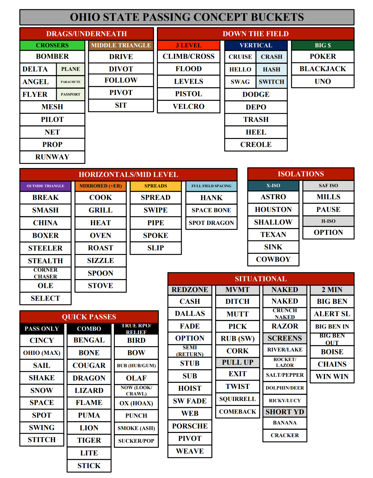
The Drags/Underneath bucket features two subcategories-crossers and middle triangle. Crossers plays are mesh variations and all flight themed. For example, net is mesh out of 3x1 combined with the popular quarters beater “mills” concept:

Delta, Angel, and Flyer are all mesh variations that create middle triangle spacing with the rail, sit, and shallow. They are all grouped into a further subcategory along with the mesh return constraint play off of the same look. For example, Delta is mesh with middle triangle spacing:

Plane is grouped with and right across from Delta and is simply the mesh return variation of the same play:

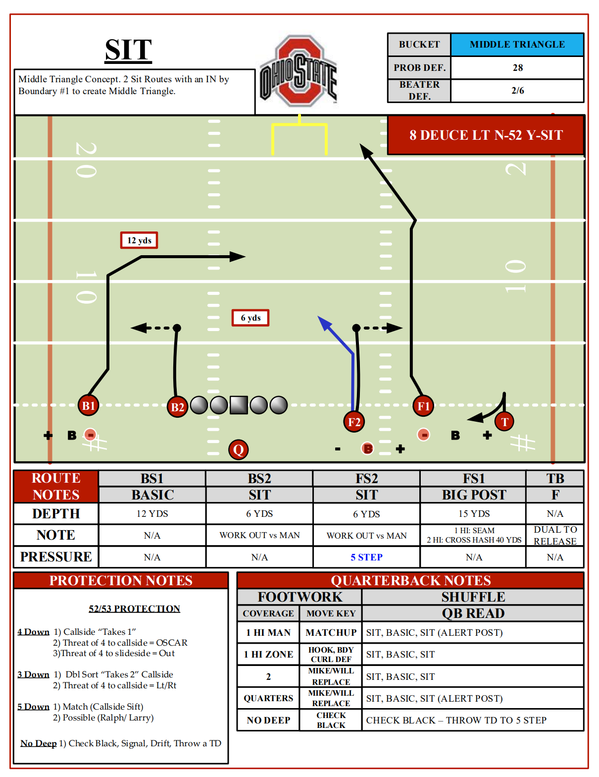
The middle triangles category are passing concepts that create a middle triangle within the underneath portion of the defense. An example is “Sit”:
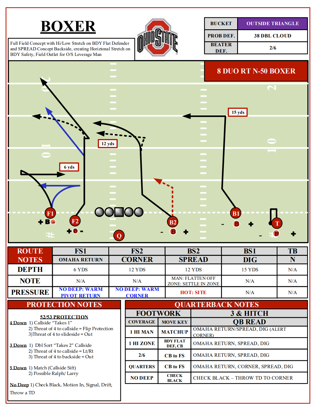
For those well versed in football terminology, most of these buckets are self-explanatory. However, there isn’t necessarily a ubiquitous understanding of what concepts would fall under the category of “outside triangle” in football. Ohio State designates this passing game family as one that places a vertical stretch on the boundary flat defender and a horizontal stretch on the boundary safety. It is what most would consider smash to the boundary and Y cross from the field. A good example from the outside triangle bucket is “Boxer”:
Once all of the concepts they will use for a given year are established, they organize and place them as magnets on a whiteboard. When game planning, they can visualize the full spectrum of the offense and move the magnets/plays over that they want to use for that week. To help them streamline the process of deciding which pass plays to run in a given week, they create a spreadsheet in the off season of the entire passing game and how each individual pass play matches up against every coverage they’ve seen-a total of 21 different coverages. The pass plays are grouped by bucket and are placed on the Y axis, while coverages are placed on the X axis. Green indicates that the pass play is efficient vs a specific coverage:

Before the coaches come in on Monday to start game planning, a member of the staff takes the spreadsheet and filters it down to the anticipated coverages they will see that week:

Now when they meet on a Monday, the lion share of work has been done in the off season (one side note is that this picture is from the clinic, which was done in 2022, so by this point they have changed their themes and play names from what they were in 2019). It is easy for them to visualize and see which pass plays they should select that have the best chance of success against the specific coverages they are anticipating from their opponent. This reminded me a bit of the Tony Franklin System “best play calls by coverage” spreadsheet I came across a few years ago:

Once a pass play has been selected, they then select the specific variation of that play that they are going to use for that week. They do this by selecting from the compendium made in the off season that features a diagram of every way they have run that specific play over the years:
As far as the total volume of plays they want to have for the game plan in a given week, they will refer to their calls by situation chart, which breaks down the average number of plays for each situation they will have in a game-a total of 75 plays:

This doesn’t mean they will carry exactly 75 plays into the game plan, but it gives them a ballpark number to refer to. So for example, the chart shows that they will, on average, encounter a 3rd and long situation 3 times. Day will carry 5 third and long calls into a game. The entire process of bucket organization, spreadsheets, catalogs, and charts that they utilize are all designed for one reason-efficiency. As Day explained at the clinic, “You have what you need, you are not wasting time running and practicing plays that you are not going to get to. You want to have answers, but you want to have plays that your guys can actually execute.”
Day’s calls by situation chart brought to my mind the excellent book former Ravens head coach Brian Billick wrote back in the 1990’s, specifically the portion where he addresses the question of how much offense an OC should carry into the game plan. In true form as a Bill Walsh protege, Billick’s process for determining offensive volume is laid out by the numbers and in extreme detail in the first chapter. I will summarize his process and try to highlight certain points that I think can apply to any offensive coordinator.
According to Billick, the two questions that first must be answered when determining offensive volume are:
How much offense can my team run during a season?
How much offense can be effectively practiced and run each week?
The amount of offense one can carry must be thought of on 3 levels-yearly, weekly, and game day. Your goal should be to have a great amount of overlap between your total offensive volume and the amount of offense you can effectively practice. There are of course a variety of situations you could encounter in any given game that force you to carry certain plays into a game that you never end up using. Billick explains his thought process when it comes to this non-negotiable aspect of the game plan he refers to as “overage”:
It is impossible to accurately predict the exact amount of offense you will use in any given game. There is always going to be a certain amount of overage that has to be built in for the “what if’s”. For example, “what if” they blitz more than you had thought?; “what if” you aren’t able to run the ball as well as you thought?; “what if” your quarterback is having an off day?; or “what if” the weather is bad? We have tried to keep our overage to between 25-30 percent of the total game snaps we can predict. This percentage of overage is something we work very hard to maintain. Each week, I examine how much of the offensive game plan was actually used vs. what was installed and practiced, looking to see if our offensive game plan can be pared down. On the other hand, you have to be careful about not limiting yourself too much. Many coaches may try to eliminate too much offense because it makes less for them to have to prepare. You don’t want to waste time working on things you are never going to use, but you must have all that you need to get the job done.
Bilick then goes on to provide diagrams that illustrate various offensive game plans and actual game play ratios.

Diagram 1-2 represents a balanced 50/50 ratio between the run and the pass type of offensive system. The game plan and actual game day calls fell within what was expected going into the game. As Billick puts it, “This situation is obviously a winning profile when the amount of offense practiced and used match each other very well.”

Diagrams 1-3 and 1-4 represent the same offensive system but a different game plan. In this scenario, the game plan featured a higher volume of pass plays to attack the defense’s weak point-the secondary. In diagram 1-3, the game went according to plan. In diagram 1-4, the offense had the same game plan but discovered during the game that they were able to run the ball much more effectively than they had anticipated and ended up calling more run plays. “Both examples showed you planned well, were very efficient in your preparation, and were able to stay with your basic game plan.”

Diagrams 1-5 and 1-6 display a game plan focused heavier on the run for that week. Diagram 1-5 fell within the expected parameters, while diagram 1-6 shows a team that had to draw from their passing game far more predominantly than they planned for, even having to run pass plays from their offensive system that they did not practice during the week. Billick explains that “ideally, you would like to keep this type of play calling to a minimum. Often, however, there may be a base part of your attack that you have used enough during the year that even though you may not have emphasized it during the week, you are still comfortable coming back to it in any given game.”

Diagrams 1-7 and 1-8 illustrate a team whose offensive system is run dominant. Diagram 1-7 shows a game plan that was well executed, showing game day calls fell within expected parameters. Diagram 1-8 is indicative of a disastrous day for the offense, with the play caller using mostly pass plays and drawing not only from their pass game that wasn’t practiced that week, but also making up plays during the game. This is a worst case scenario type of situation that can be entirely avoided if the game planning process is done correctly.

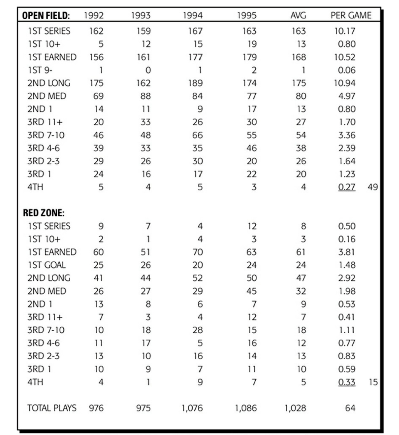
When determining the number of plays for your offense on the 3 levels mentioned earlier-yearly, weekly, and on game day, Billick explains that those parameters should be determined based on the actual numbers of plays in a game and the number of various situations in which you will be using those plays. The barometer he would use for determining the size and scope of his offense would be based on NFL averages as well as the averages for his own team from previous years. The figure below displays the averages for his Vikings teams during the 1992-1995 seasons for play calls dealing with open field and red zone situations. The total number of plays of average plays in a game was 64:
College rules allow for a higher number of average plays per game. For example, in the 3 years before Bill Walsh took over at Stanford, the team averaged 72 plays per game (this is almost certainly one of the charts Walsh used when he first started planning out his offense for the college game when he took over at Stanford in 1992):

These averages are similar to the call by situations chart mentioned previously that Ryan Day (75 total plays) uses to determine offensive capacity. As is the case with statistics, Billick explains in his book that there are of course fluctuations in these numbers in any given game, but they are certainly a good starting point in deciding the amount of offense that you need. As he points out at the end of the chapter, “The averages in each area can help us set the parameters for the size of the offensive package we need and ultimately the amount of offense we will use in a week. These numbers stay amazingly consistent from year to year and even from team to team.”
The famous quote by Abraham Lincoln, “Give me 8 hours to chop down a tree, and I will spend 6 of them sharpening my axe” can certainly be applied to constructing an offense. Careful strategizing in regards to the size and scope of your offensive system is paramount to success. Having a detailed plan and process in place to determine offensive volume will maximize the efficiency of your offense on game day.